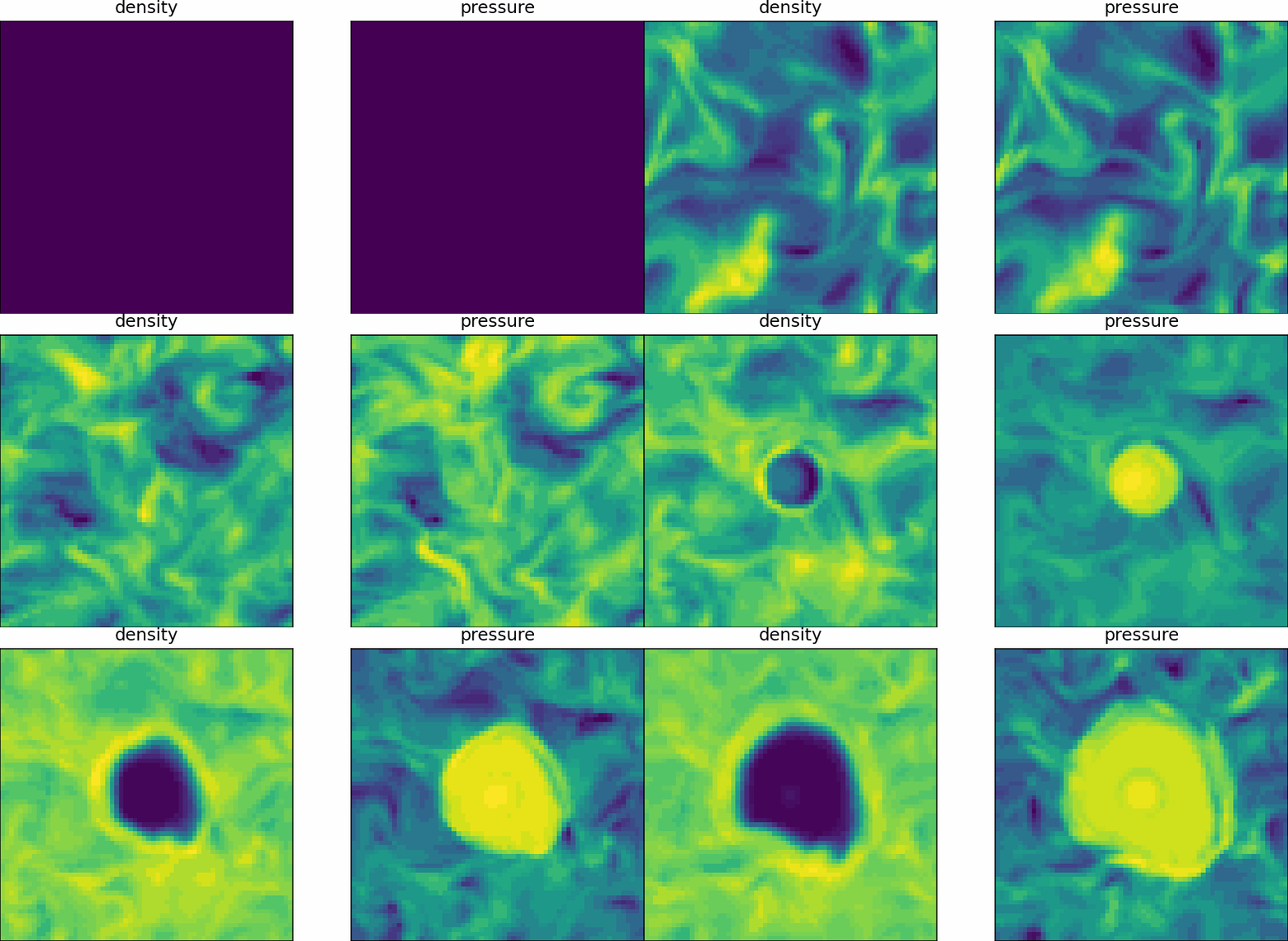
astronomix MHD example - stellar wind in the turbulent ISM

Let us simulate stellar wind in the turbulent ISM :) At \(64^3\) cells the whole notebook should complete a few minutes :D

Hint: Make sure to run on GPU.

Imports

# ==== GPU selection ====
from autocvd import autocvd
autocvd(num_gpus = 1)
# ruff: noqa: E402
# =======================

import jax
import jax.numpy as jnp
import os
import re

# astronomix constants
from astronomix import (
    FINITE_DIFFERENCE,
    PERIODIC_BOUNDARY,
)

# astronomix containers
from astronomix import (
    SimulationConfig,
    PositivityConfig,
    BoundarySettings,
    BoundarySettings1D,
    SimulationParams,
    WindParams,
    CodeUnits,
)
from astronomix.option_classes import WindConfig
from astronomix._modules._turbulent_forcing._turbulent_forcing_options import (
    TurbulentForcingConfig,
    TurbulentForcingParams,
)

# astronomix functions
from astronomix import (
    get_registered_variables,
    get_helper_data,
    construct_primitive_state,
    time_integration,
    initialize_interface_fields,
    finalize_config,
)

# units
from astropy import units as u
import astropy.constants as c

# plotting
import matplotlib.pyplot as plt
from matplotlib.colors import LogNorm
import imageio.v3 as iio
from IPython.display import Image

Simulation setup

# simulation settings
gamma = 5/3

# spatial domain
box_size = 1.0
num_cells = 64

# activate stellar wind
stellar_wind = False

# turbulence
turbulence = True

# otherwise B = 0.0
mhd = True

app_string = "driven_turb_wind"

# baseline simulation config
config = SimulationConfig(
    solver_mode = FINITE_DIFFERENCE,
    mhd = True,
    progress_bar = True,
    positivity_config = PositivityConfig(default_positivity_protection = True),
    donate_state = True, # save storage
    dimensionality = 3,
    box_size = box_size,
    num_cells = num_cells,
    turbulent_forcing_config = TurbulentForcingConfig(
        turbulent_forcing = turbulence,
    ),
    boundary_settings =  BoundarySettings(
        BoundarySettings1D(
            left_boundary = PERIODIC_BOUNDARY,
            right_boundary = PERIODIC_BOUNDARY
        ),
        BoundarySettings1D(
            left_boundary = PERIODIC_BOUNDARY,
            right_boundary = PERIODIC_BOUNDARY
        ),
        BoundarySettings1D(
            left_boundary = PERIODIC_BOUNDARY,
            right_boundary = PERIODIC_BOUNDARY
        )
    ),
    # animation
    activate_snapshot_callback = True,
    num_snapshots = 100
)

# get the variable registry
registered_variables = get_registered_variables(config)

# unit setup
code_length = 3 * u.parsec
code_mass = 1 * u.M_sun
code_velocity = 100 * u.km / u.s
code_units = CodeUnits(code_length, code_mass, code_velocity)

# time domain
C_CFL = 0.8

# wind parameters
M_star = 40 * u.M_sun
wind_final_velocity = 2000 * u.km / u.s
wind_mass_loss_rate = 2.965e-3 / (1e6 * u.yr) * M_star

wind_params = WindParams(
    wind_mass_loss_rate = wind_mass_loss_rate.to(code_units.code_mass / code_units.code_time).value,
    wind_final_velocity = wind_final_velocity.to(code_units.code_velocity).value
)

params = SimulationParams(
    C_cfl = C_CFL,
    dt_max = 0.1,
    gamma = gamma,
    minimum_density=1e-3,
    minimum_pressure=1e-3,
    wind_params = wind_params,
    turbulent_forcing_params = TurbulentForcingParams(
        energy_injection_rate = 0.2
    ),
)

print((0.2 * code_units.code_energy / code_units.code_time).to(u.erg / u.s))

# homogeneous initial state
rho_0 = 2 * c.m_p / u.cm**3
p_0 = 3e4 * u.K / u.cm**3 * c.k_B

rho = jnp.ones((config.num_cells, config.num_cells, config.num_cells)) * rho_0.to(code_units.code_density).value
u_x = jnp.zeros((config.num_cells, config.num_cells, config.num_cells))
u_y = jnp.zeros((config.num_cells, config.num_cells, config.num_cells))
u_z = jnp.zeros((config.num_cells, config.num_cells, config.num_cells))
p = jnp.ones((config.num_cells, config.num_cells, config.num_cells)) * p_0.to(code_units.code_pressure).value

if mhd:
    B_0 = 13.5 * u.microgauss / c.mu0**0.5
    B_0 = B_0.to(code_units.code_magnetic_field).value
else:
    B_0 = 0.0

B_x = jnp.ones((config.num_cells, config.num_cells, config.num_cells)) * B_0
B_y = jnp.zeros((config.num_cells, config.num_cells, config.num_cells))
B_z = jnp.zeros((config.num_cells, config.num_cells, config.num_cells))
bxb, byb, bzb = initialize_interface_fields(B_x, B_y, B_z)

# construct primitive state
initial_state = construct_primitive_state(
    config = config,
    registered_variables=registered_variables,
    density = rho,
    velocity_x = u_x,
    velocity_y = u_y,
    velocity_z = u_z,
    gas_pressure = p,
    magnetic_field_x = B_x,
    magnetic_field_y = B_y,
    magnetic_field_z = B_z,
    interface_magnetic_field_x = bxb,
    interface_magnetic_field_y = byb,
    interface_magnetic_field_z = bzb,
)

config = finalize_config(config, initial_state.shape)

4.295998351923327e+34 erg / s
OPTIMAL_BACKEND: using the PALLAS backend (GPU compute capability >= 8.0).
For 3D simulations with periodic boundaries, setting boundary handling to PERIODIC_ROLL and num_ghost_cells to 0 for better performance.
Setting time integrator to RK4_SSP for finite difference solver mode.

Prepare saving frames for GIF

import os

# create folder for frames
os.makedirs('turb_frames', exist_ok=True)
os.makedirs('wind_frames', exist_ok=True)

# empty the folders
for filename in os.listdir('turb_frames'):
  os.remove(os.path.join('turb_frames', filename))
for filename in os.listdir('wind_frames'):
  os.remove(os.path.join('wind_frames', filename))

def save_frame(
  time,
  state,
  registered_variables,
  directory
):

  def plot_slices(density, pressure, time):

    print(f"plotting slice at t = {time}")

    fig, (ax1, ax3) = plt.subplots(1, 2, figsize=(8, 4))

    # equal aspect ratio
    ax1.set_aspect('equal', 'box')
    # ax2.set_aspect('equal', 'box')
    ax3.set_aspect('equal', 'box')

    # remove x and y ticks
    for ax in [ax1, ax3]:
      ax.set_xticks([])
      ax.set_yticks([])

    z_level = num_cells // 2

    im1 = ax1.imshow(density.T, origin = "lower", extent = [0, 1, 0, 1], norm = LogNorm())
    ax1.set_title("density")

    # im2 = ax2.imshow(velocity.T, origin = "lower", extent = [0, 1, 0, 1])
    # ax2.set_title("velocity magnitude")

    im3 = ax3.imshow(pressure.T, origin = "lower", extent = [0, 1, 0, 1], norm = LogNorm())
    ax3.set_title("pressure")

    fig.savefig(
      f"{directory}/frame{time}.png",
      dpi=150,
      bbox_inches="tight",
      pad_inches=0
    )

    plt.close(fig)

  num_vars, nx, ny, nz = state.shape
  z_level = num_cells // 2

  density = state[registered_variables.density_index, :, :, z_level]
  # velocity = jnp.sqrt(state[registered_variables.velocity_index.x, :, :, z_level]**2 + state[registered_variables.velocity_index.y, :, :, z_level]**2 + state[registered_variables.velocity_index.z, :, :, z_level]**2)
  pressure = state[registered_variables.pressure_index, :, :, z_level]

  jax.debug.callback(
      plot_slices,
      density, pressure, time,
  )

save_turb_frame = lambda time, state, registered_variables: save_frame(time, state, registered_variables, 'turb_frames')
save_wind_frame = lambda time, state, registered_variables: save_frame(time, state, registered_variables, 'wind_frames')

Turbulence only run

Parameter adaptation

t_final = 6.0 * 1e4 * u.yr
t_end = t_final.to(code_units.code_time).value

# set the final time
params = params._replace(
    t_end = t_end,
)

Running the simulation

turb_state = time_integration(initial_state, config, params, registered_variables, save_turb_frame)

plotting slice at t = 0.0
plotting slice at t = 0.0283597931265831--------------------------------| 1.4%  
plotting slice at t = 0.04713613539934158-------------------------------| 2.3%  
plotting slice at t = 0.06446469575166702-------------------------------| 3.2%  
plotting slice at t = 0.0879751518368721--------------------------------| 4.3%  
plotting slice at t = 0.1028243824839592--------------------------------| 5.0%  
plotting slice at t = 0.12407807260751724-------------------------------| 6.1%  
plotting slice at t = 0.14407825469970703-------------------------------| 7.0%  
plotting slice at t = 0.16847829520702362-------------------------------| 8.2%  
plotting slice at t = 0.18567919731140137-------------------------------| 9.1%  
plotting slice at t = 0.2088324874639511-------------------------------| 10.2%  
plotting slice at t = 0.22603651881217957------------------------------| 11.1%  
plotting slice at t = 0.24801519513130188------------------------------| 12.1%  
plotting slice at t = 0.26925113797187805------------------------------| 13.2%  
plotting slice at t = 0.2890871465206146-------------------------------| 14.1%  
plotting slice at t = 0.30821502208709717------------------------------| 15.1%  
plotting slice at t = 0.3319496810436249-------------------------------| 16.2%  
plotting slice at t = 0.35032910108566284------------------------------| 17.1%  
plotting slice at t = 0.36885154247283936------------------------------| 18.0%  
plotting slice at t = 0.391033411026001--------------------------------| 19.1%  
plotting slice at t = 0.4120686650276184-------------------------------| 20.1%  
plotting slice at t = 0.4324694573879242-------------------------------| 21.1%  
plotting slice at t = 0.4521752595901489-------------------------------| 22.1%  
plotting slice at t = 0.47145116329193115------------------------------| 23.0%  
plotting slice at t = 0.4941686987876892-------------------------------| 24.2%  
plotting slice at t = 0.5133548378944397-------------------------------| 25.1%  
plotting slice at t = 0.531941831111908--------------------------------| 26.0%  
plotting slice at t = 0.5535133481025696-------------------------------| 27.1%  
plotting slice at t = 0.5752507448196411-------------------------------| 28.1%  
plotting slice at t = 0.5965901613235474-------------------------------| 29.2%  
plotting slice at t = 0.6142207980155945-------------------------------| 30.0%  
plotting slice at t = 0.6352341771125793-------------------------------| 31.1%  
plotting slice at t = 0.655948281288147--------------------------------| 32.1%  
plotting slice at t = 0.6757218837738037-------------------------------| 33.0%  
plotting slice at t = 0.6986491680145264-------------------------------| 34.2%  
plotting slice at t = 0.7182086110115051-------------------------------| 35.1%  
plotting slice at t = 0.7368654608726501-------------------------------| 36.0%  
plotting slice at t = 0.7578786611557007-------------------------------| 37.1%  
plotting slice at t = 0.7788305282592773-------------------------------| 38.1%  
plotting slice at t = 0.7988430261611938-------------------------------| 39.1%  
plotting slice at t = 0.8188855648040771-------------------------------| 40.0%  
plotting slice at t = 0.8386537432670593-------------------------------| 41.0%  
plotting slice at t = 0.8607021570205688-------------------------------| 42.1%  
plotting slice at t = 0.8797156810760498-------------------------------| 43.0%  
plotting slice at t = 0.9013005495071411-------------------------------| 44.1%  
plotting slice at t = 0.9223417639732361-------------------------------| 45.1%  
plotting slice at t = 0.9433245062828064-------------------------------| 46.1%  
plotting slice at t = 0.9638853669166565-------------------------------| 47.1%  
plotting slice at t = 0.9820597767829895-------------------------------| 48.0%  
plotting slice at t = 1.0026311874389648-------------------------------| 49.0%  
plotting slice at t = 1.0228747129440308-------------------------------| 50.0%  
plotting slice at t = 1.045531988143921--------------------------------| 51.1%  
plotting slice at t = 1.06522536277771---------------------------------| 52.1%  
plotting slice at t = 1.0844675302505493-------------------------------| 53.0%  
plotting slice at t = 1.1048825979232788-------------------------------| 54.0%  
plotting slice at t = 1.12700355052948██-------------------------------| 55.1%  
plotting slice at t = 1.1454445123672485-------------------------------| 56.0%  
plotting slice at t = 1.1672405004501343█------------------------------| 57.1%  
plotting slice at t = 1.188157081604004███-----------------------------| 58.1%  
plotting slice at t = 1.2071654796600342██-----------------------------| 59.0%  
plotting slice at t = 1.22748863697052█████----------------------------| 60.0%  
plotting slice at t = 1.2487962245941162████---------------------------| 61.1%  
plotting slice at t = 1.2685893774032593████---------------------------| 62.0%  
plotting slice at t = 1.2903856039047241█████--------------------------| 63.1%  
plotting slice at t = 1.3107597827911377██████-------------------------| 64.1%  
plotting slice at t = 1.3308385610580444██████-------------------------| 65.1%  
plotting slice at t = 1.350176453590393████████------------------------| 66.0%  
plotting slice at t = 1.3717318773269653████████-----------------------| 67.1%  
plotting slice at t = 1.3915499448776245████████-----------------------| 68.0%  
plotting slice at t = 1.4122823476791382█████████----------------------| 69.0%  
plotting slice at t = 1.432869791984558███████████---------------------| 70.1%  
plotting slice at t = 1.4524978399276733██████████---------------------| 71.0%  
plotting slice at t = 1.4741660356521606███████████--------------------| 72.1%  
plotting slice at t = 1.4942288398742676████████████-------------------| 73.1%  
plotting slice at t = 1.5150158405303955█████████████------------------| 74.1%  
plotting slice at t = 1.534738302230835██████████████------------------| 75.0%  
plotting slice at t = 1.5551702976226807██████████████-----------------| 76.0%  
plotting slice at t = 1.575640320777893████████████████----------------| 77.0%  
plotting slice at t = 1.5955696105957031███████████████----------------| 78.0%  
plotting slice at t = 1.6163556575775146████████████████---------------| 79.0%  
plotting slice at t = 1.637665033340454██████████████████--------------| 80.1%  
plotting slice at t = 1.6574229001998901█████████████████--------------| 81.0%  
plotting slice at t = 1.678769588470459███████████████████-------------| 82.1%  
plotting slice at t = 1.6983786821365356███████████████████------------| 83.0%  
plotting slice at t = 1.7189027070999146███████████████████------------| 84.0%  
plotting slice at t = 1.7393792867660522████████████████████-----------| 85.0%  
plotting slice at t = 1.7605520486831665█████████████████████----------| 86.1%  
plotting slice at t = 1.7808797359466553██████████████████████---------| 87.1%  
plotting slice at t = 1.8004584312438965██████████████████████---------| 88.0%  
plotting slice at t = 1.8220678567886353███████████████████████--------| 89.1%  
plotting slice at t = 1.8412578105926514████████████████████████-------| 90.0%  
plotting slice at t = 1.862190842628479█████████████████████████-------| 91.0%  
plotting slice at t = 1.8824282884597778█████████████████████████------| 92.0%  
plotting slice at t = 1.9026882648468018██████████████████████████-----| 93.0%  
plotting slice at t = 1.9239016771316528██████████████████████████-----| 94.1%  
plotting slice at t = 1.944503664970398████████████████████████████----| 95.1%  
plotting slice at t = 1.964837908744812█████████████████████████████---| 96.1%  
plotting slice at t = 1.9849492311477661████████████████████████████---| 97.0%  
plotting slice at t = 2.0061283111572266█████████████████████████████--| 98.1%  
plotting slice at t = 2.025508403778076███████████████████████████████-| 99.0%  
 |████████████████████████████████████████████████████████████████████| 100.0%  
plotting slice at t = 2.045424222946167

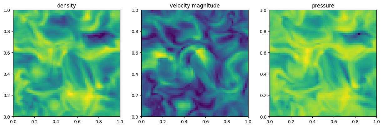
Plotting

fig, (ax1, ax2, ax3) = plt.subplots(1, 3, figsize=(15, 5))

# equal aspect ratio
ax1.set_aspect('equal', 'box')
ax2.set_aspect('equal', 'box')
ax3.set_aspect('equal', 'box')

z_level = num_cells // 2

ax1.imshow(turb_state[registered_variables.density_index, :, :, z_level].T, origin = "lower", extent = [0, 1, 0, 1], norm = LogNorm())
ax1.set_title("density")

ax2.imshow(jnp.sqrt(turb_state[registered_variables.velocity_index.x, :, :, z_level]**2 + turb_state[registered_variables.velocity_index.y, :, :, z_level]**2 + turb_state[registered_variables.velocity_index.z, :, :, z_level]**2).T, origin = "lower", extent = [0, 1, 0, 1])
ax2.set_title("velocity magnitude")

ax3.imshow(turb_state[registered_variables.pressure_index, :, :, z_level].T, origin = "lower", extent = [0, 1, 0, 1], norm = LogNorm())
ax3.set_title("pressure")

Text(0.5, 1.0, 'pressure')

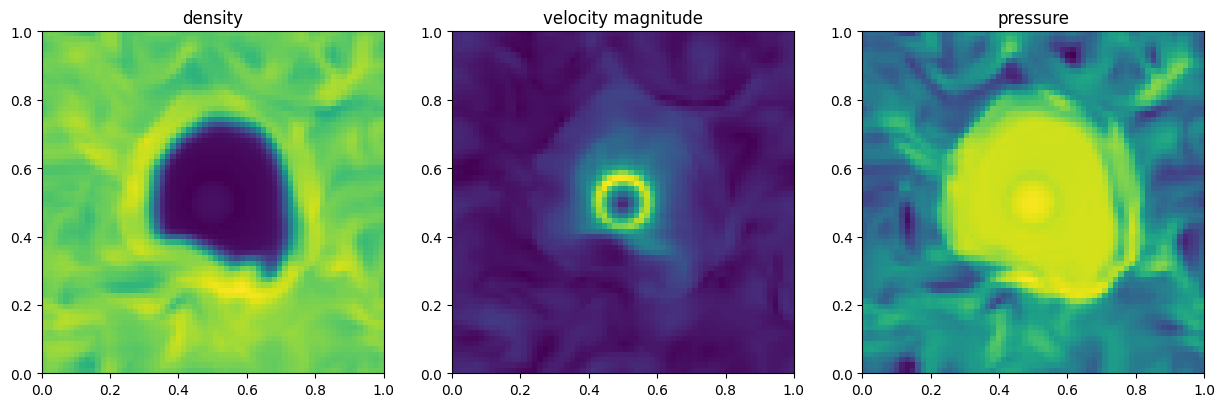
Let us introduce stellar wind

Parameter adaptation

# then stellar wind + turbulence
t_final = 0.5 * 1e4 * u.yr
t_end = t_final.to(code_units.code_time).value
print(t_end)
config = config._replace(
    wind_config = WindConfig(
        stellar_wind = True,
        num_injection_cells = 4,
    ),
)
params = params._replace(
    t_end = t_end,
    minimum_density = 1e-3,
    minimum_pressure = 1e-3,
)

0.17045202750761582

Running the simulation

final_state = time_integration(turb_state, config, params, registered_variables, save_wind_frame)

plotting slice at t = 0.0
plotting slice at t = 0.0019810188096016645-----------------------------| 1.2%  
plotting slice at t = 0.0038320347666740417-----------------------------| 2.2%  
plotting slice at t = 0.005379598122090101------------------------------| 3.2%  
plotting slice at t = 0.008022702299058437------------------------------| 4.7%  
plotting slice at t = 0.009201617911458015------------------------------| 5.4%  
plotting slice at t = 0.010303299874067307------------------------------| 6.0%  
plotting slice at t = 0.012289786711335182------------------------------| 7.2%  
plotting slice at t = 0.014082222245633602------------------------------| 8.3%  
plotting slice at t = 0.015736715868115425------------------------------| 9.2%  
plotting slice at t = 0.017279885709285736-----------------------------| 10.1%  
plotting slice at t = 0.01944713294506073------------------------------| 11.4%  
plotting slice at t = 0.020814938470721245-----------------------------| 12.2%  
plotting slice at t = 0.02279547043144703------------------------------| 13.4%  
plotting slice at t = 0.024068612605333328-----------------------------| 14.1%  
plotting slice at t = 0.025922929868102074-----------------------------| 15.2%  
plotting slice at t = 0.027726415544748306-----------------------------| 16.3%  
plotting slice at t = 0.02950163371860981------------------------------| 17.3%  
plotting slice at t = 0.031243201345205307-----------------------------| 18.3%  
plotting slice at t = 0.032391373068094254-----------------------------| 19.0%  
plotting slice at t = 0.03464947268366814------------------------------| 20.3%  
plotting slice at t = 0.03632330894470215------------------------------| 21.3%  
plotting slice at t = 0.03799383342266083------------------------------| 22.3%  
plotting slice at t = 0.03966129943728447------------------------------| 23.3%  
plotting slice at t = 0.04131921008229256------------------------------| 24.2%  
plotting slice at t = 0.042970601469278336-----------------------------| 25.2%  
plotting slice at t = 0.044609494507312775-----------------------------| 26.2%  
plotting slice at t = 0.04623023793101311------------------------------| 27.1%  
plotting slice at t = 0.04783298820257187------------------------------| 28.1%  
plotting slice at t = 0.04992392286658287------------------------------| 29.3%  
plotting slice at t = 0.05145123600959778------------------------------| 30.2%  
plotting slice at t = 0.05294360965490341------------------------------| 31.1%  
plotting slice at t = 0.05486980080604553------------------------------| 32.2%  
plotting slice at t = 0.056267254054546356-----------------------------| 33.0%  
plotting slice at t = 0.05807463079690933------------------------------| 34.1%  
plotting slice at t = 0.05982620641589165------------------------------| 35.1%  
plotting slice at t = 0.06152714788913727------------------------------| 36.1%  
plotting slice at t = 0.06317972391843796------------------------------| 37.1%  
plotting slice at t = 0.06478584557771683------------------------------| 38.0%  
plotting slice at t = 0.06673083454370499------------------------------| 39.1%  
plotting slice at t = 0.06824354082345963------------------------------| 40.0%  
plotting slice at t = 0.07008658349514008------------------------------| 41.1%  
plotting slice at t = 0.07188024371862411------------------------------| 42.2%  
plotting slice at t = 0.07363420724868774------------------------------| 43.2%  
plotting slice at t = 0.07500973343849182------------------------------| 44.0%  
plotting slice at t = 0.07703228294849396------------------------------| 45.2%  
plotting slice at t = 0.07868559658527374------------------------------| 46.2%  
plotting slice at t = 0.08031472563743591------------------------------| 47.1%  
plotting slice at t = 0.08192139118909836------------------------------| 48.1%  
plotting slice at t = 0.08382145315408707------------------------------| 49.2%  
plotting slice at t = 0.08538288623094559------------------------------| 50.1%  
plotting slice at t = 0.08723392337560654------------------------------| 51.2%  
plotting slice at t = 0.08876089751720428------------------------------| 52.1%  
plotting slice at t = 0.09057136625051498------------------------------| 53.1%  
plotting slice at t = 0.09206788241863251------------------------------| 54.0%  
plotting slice at t = 0.09385272860527039------------------------------| 55.1%  
plotting slice at t = 0.0956239327788353-------------------------------| 56.1%  
plotting slice at t = 0.09738393127918243------------------------------| 57.1%  
plotting slice at t = 0.09913620352745056█-----------------------------| 58.2%  
plotting slice at t = 0.10058938711881638█-----------------------------| 59.0%  
plotting slice at t = 0.10232562571763992██----------------------------| 60.0%  
plotting slice at t = 0.10405614227056503███---------------------------| 61.0%  
plotting slice at t = 0.10578147321939468███---------------------------| 62.1%  
plotting slice at t = 0.10750395804643631████--------------------------| 63.1%  
plotting slice at t = 0.10922516882419586█████-------------------------| 64.1%  
plotting slice at t = 0.11094110459089279█████-------------------------| 65.1%  
plotting slice at t = 0.11264894157648087██████------------------------| 66.1%  
plotting slice at t = 0.11434682458639145███████-----------------------| 67.1%  
plotting slice at t = 0.11603907495737076███████-----------------------| 68.1%  
plotting slice at t = 0.11772634088993073████████----------------------| 69.1%  
plotting slice at t = 0.11940908432006836█████████---------------------| 70.1%  
plotting slice at t = 0.1210901066660881███████████--------------------| 71.0%  
plotting slice at t = 0.12276691943407059██████████--------------------| 72.0%  
plotting slice at t = 0.12443944811820984███████████-------------------| 73.0%  
plotting slice at t = 0.12638509273529053████████████------------------| 74.1%  
plotting slice at t = 0.12804998457431793████████████------------------| 75.1%  
plotting slice at t = 0.12970933318138123█████████████-----------------| 76.1%  
plotting slice at t = 0.131364643573761████████████████----------------| 77.1%  
plotting slice at t = 0.13302011787891388██████████████----------------| 78.0%  
plotting slice at t = 0.1346758008003235████████████████---------------| 79.0%  
plotting slice at t = 0.1366027444601059█████████████████--------------| 80.1%  
plotting slice at t = 0.1382504552602768█████████████████--------------| 81.1%  
plotting slice at t = 0.1398957222700119██████████████████-------------| 82.1%  
plotting slice at t = 0.14154155552387238██████████████████------------| 83.0%  
plotting slice at t = 0.14318639039993286██████████████████------------| 84.0%  
plotting slice at t = 0.14510592818260193███████████████████-----------| 85.1%  
plotting slice at t = 0.14674879610538483████████████████████----------| 86.1%  
plotting slice at t = 0.14838525652885437█████████████████████---------| 87.1%  
plotting slice at t = 0.1500253528356552██████████████████████---------| 88.0%  
plotting slice at t = 0.15193703770637512██████████████████████--------| 89.1%  
plotting slice at t = 0.15357397496700287███████████████████████-------| 90.1%  
plotting slice at t = 0.15520672500133514███████████████████████-------| 91.1%  
plotting slice at t = 0.15683090686798096████████████████████████------| 92.0%  
plotting slice at t = 0.15872032940387726█████████████████████████-----| 93.1%  
plotting slice at t = 0.1603388488292694██████████████████████████-----| 94.1%  
plotting slice at t = 0.1619555950164795███████████████████████████----| 95.0%  
plotting slice at t = 0.16384045779705048███████████████████████████---| 96.1%  
plotting slice at t = 0.16545335948467255███████████████████████████---| 97.1%  
plotting slice at t = 0.1670646220445633█████████████████████████████--| 98.0%  
plotting slice at t = 0.16894084215164185█████████████████████████████-| 99.1%  
 |████████████████████████████████████████████████████████████████████| 100.0%  
plotting slice at t = 0.1704520285129547

Plotting

fig, (ax1, ax2, ax3) = plt.subplots(1, 3, figsize=(15, 5))

# equal aspect ratio
ax1.set_aspect('equal', 'box')
ax2.set_aspect('equal', 'box')
ax3.set_aspect('equal', 'box')

z_level = num_cells // 2

ax1.imshow(final_state[registered_variables.density_index, :, :, z_level].T, origin = "lower", extent = [0, 1, 0, 1], norm = LogNorm())
ax1.set_title("density")

ax2.imshow(jnp.sqrt(final_state[registered_variables.velocity_index.x, :, :, z_level]**2 + final_state[registered_variables.velocity_index.y, :, :, z_level]**2 + final_state[registered_variables.velocity_index.z, :, :, z_level]**2).T, origin = "lower", extent = [0, 1, 0, 1])
ax2.set_title("velocity magnitude")

ax3.imshow(final_state[registered_variables.pressure_index, :, :, z_level].T, origin = "lower", extent = [0, 1, 0, 1], norm = LogNorm())
ax3.set_title("pressure")

Text(0.5, 1.0, 'pressure')

Make animations

def get_sorted_frames(directory):
    files = [f for f in os.listdir(directory) if f.endswith('.png')]
    # Extract numerical timestamp from filename (e.g., frame0.123.png -> 0.123)
    # and sort by it
    files.sort(key=lambda f: float(re.search(r'frame([0-9.]+)\.png', f).group(1)))
    return [os.path.join(directory, f) for f in files]

turb_frames = get_sorted_frames('turb_frames')
wind_frames = get_sorted_frames('wind_frames')

all_frames = turb_frames + wind_frames

# Read all images into a list
images = [iio.imread(frame) for frame in all_frames]

# Create GIF
gif_path = 'simulation_animation.gif'
iio.imwrite(gif_path, images, duration=int(1000/30), loop=0)

print(f"GIF created at: {gif_path}")

GIF created at: simulation_animation.gif

No check the gif created under the files tab (simulation_animation.gif) :)

Image(filename='simulation_animation.gif')