Field Level Inference with Target Projections

Imports

# ==== GPU selection ====
from autocvd import autocvd
autocvd(num_gpus = 1)
# ruff: noqa: E402
# =======================

# general
import jax
import jax.numpy as jnp
import optax

# astronomix constants
from astronomix import (
    FINITE_DIFFERENCE,
    FINITE_VOLUME,
    PERIODIC_BOUNDARY,
    BACKWARDS,
)

# astronomix containers
from astronomix import (
    SimulationConfig,
    PositivityConfig,
    BoundarySettings,
    BoundarySettings1D,
    SimulationParams,
    CodeUnits,
)
from astronomix._modules._turbulent_forcing._turbulent_forcing_options import (
    TurbulentForcingConfig,
    TurbulentForcingParams,
)

# astronomix functions
from astronomix import (
    get_registered_variables,
    get_helper_data,
    construct_primitive_state,
    time_integration,
    initialize_interface_fields,
    finalize_config,
)

# units
from astropy import units as u
import astropy.constants as c

# plotting
import matplotlib.pyplot as plt
from matplotlib.colors import LogNorm
import numpy as np
import pyvista as pv

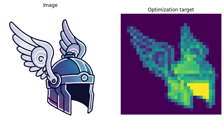
Loading the target image

resolution = 32

from PIL import Image
import jax.numpy as jnp
import matplotlib.pyplot as plt

def load_image(path, height, width, flat_profile = False):
    img = jnp.array(Image.open(path).convert("L"))
    img = 1.0 - img / 255.0 # black → 1, white → 0
    h, w = img.shape

    pad_h = (-h) % height
    pad_w = (-w) % width
    pad = ((pad_h//2, pad_h - pad_h//2),
           (pad_w//2, pad_w - pad_w//2))

    img = jnp.pad(img, pad)
    hp, wp = img.shape

    result = img.reshape(height, hp//height, width, wp//width).mean(axis=(1, 3))

    if flat_profile:
        result = jnp.where(result > 0.01, 1.01, 1.0)
    else:
        # still crunch the range between 1.01 and 1.0
        # but with all the intermediates
        result = 1.0 + (result - 0.01) / (1.0 - 0.01) * 0.01

    return result

# load the optimization target image (placed next to this notebook)
path = "logo.png"

original_rgb = Image.open(path).convert("RGB")
target = load_image(path, resolution, resolution)

fig, ax = plt.subplots(1, 2, figsize=(10, 5))

ax[0].imshow(original_rgb)
ax[0].set_title("Image")
ax[0].axis("off")

ax[1].imshow(target, cmap="viridis")
ax[1].set_title("Optimization target")
ax[1].axis("off")

(np.float64(-0.5), np.float64(31.5), np.float64(31.5), np.float64(-0.5))

Field-level inference

Generation of an initial state

# simulation settings
gamma = 5/3

# spatial domain
box_size = 1.0
num_cells = resolution

# turbulence
turbulence = True

# otherwise B = 0.0
solver_mode = FINITE_DIFFERENCE
mhd = False

# baseline simulation config
config = SimulationConfig(
    solver_mode = solver_mode,
    mhd = mhd,
    progress_bar = False,
    positivity_config = PositivityConfig(default_positivity_protection = True),
    donate_state = False, # save storage
    differentiation_mode = BACKWARDS,
    dimensionality = 3,
    box_size = box_size,
    num_cells = num_cells,
    turbulent_forcing_config = TurbulentForcingConfig(
        turbulent_forcing = turbulence,
    ),
    boundary_settings =  BoundarySettings(
        BoundarySettings1D(
            left_boundary = PERIODIC_BOUNDARY,
            right_boundary = PERIODIC_BOUNDARY
        ),
        BoundarySettings1D(
            left_boundary = PERIODIC_BOUNDARY,
            right_boundary = PERIODIC_BOUNDARY
        ),
        BoundarySettings1D(
            left_boundary = PERIODIC_BOUNDARY,
            right_boundary = PERIODIC_BOUNDARY
        )
    ),
)

# get the variable registry
registered_variables = get_registered_variables(config)

# unit setup
code_length = 3 * u.parsec
code_mass = 100 * u.M_sun
code_velocity = 100 * u.km / u.s
code_units = CodeUnits(code_length, code_mass, code_velocity)

# time domain
C_CFL = 1.5

# initial state
n_h = 2 # cm^-3
rho_0 = n_h * c.m_p / u.cm**3
p_0 = 3e4 * u.K / u.cm**3 * c.k_B

dE_dt_turb = 4.3e34 * u.erg / u.s

params = SimulationParams(
    C_cfl = C_CFL,
    dt_max = 0.1,
    gamma = gamma,
    # currently only active for the finite diff solver
    minimum_density=(1e-2 * rho_0).to(code_units.code_density).value,
    minimum_pressure=(1e-2 * p_0).to(code_units.code_pressure).value,
    turbulent_forcing_params = TurbulentForcingParams(
        energy_injection_rate = dE_dt_turb.to(code_units.code_energy / code_units.code_time).value,
    ),
)

rho = jnp.ones((config.num_cells, config.num_cells, config.num_cells)) * rho_0.to(code_units.code_density).value
u_x = jnp.zeros((config.num_cells, config.num_cells, config.num_cells))
u_y = jnp.zeros((config.num_cells, config.num_cells, config.num_cells))
u_z = jnp.zeros((config.num_cells, config.num_cells, config.num_cells))
p = jnp.ones((config.num_cells, config.num_cells, config.num_cells)) * p_0.to(code_units.code_pressure).value

if mhd:
    B_0 = 13.5 * u.microgauss / c.mu0**0.5
    B_0 = B_0.to(code_units.code_magnetic_field).value
else:
    B_0 = 0.0

B_x = jnp.ones((config.num_cells, config.num_cells, config.num_cells)) * B_0
B_y = jnp.zeros((config.num_cells, config.num_cells, config.num_cells))
B_z = jnp.zeros((config.num_cells, config.num_cells, config.num_cells))
bxb, byb, bzb = initialize_interface_fields(B_x, B_y, B_z)

# construct primitive state
initial_state = construct_primitive_state(
    config = config,
    registered_variables=registered_variables,
    density = rho,
    velocity_x = u_x,
    velocity_y = u_y,
    velocity_z = u_z,
    gas_pressure = p,
    magnetic_field_x = B_x,
    magnetic_field_y = B_y,
    magnetic_field_z = B_z,
    interface_magnetic_field_x = bxb,
    interface_magnetic_field_y = byb,
    interface_magnetic_field_z = bzb,
)

config = finalize_config(config, initial_state.shape)

t_final = 24 * 1e4 * u.yr
t_end = t_final.to(code_units.code_time).value

# set the final time
params = params._replace(
    t_end = t_end,
)

# running a small turbulent simulation
turb_state = time_integration(initial_state, config, params, registered_variables)

# calculate the rms velocity and turbulent crossing time
rms_velocity = jnp.sqrt(jnp.mean(turb_state[registered_variables.velocity_index.x]**2 + turb_state[registered_variables.velocity_index.y]**2 + turb_state[registered_variables.velocity_index.z]**2))
rms_velocity = (rms_velocity * code_units.code_velocity).to(u.km/u.s)
crossing_time = box_size * code_length / rms_velocity
print(f"RMS velocity: {rms_velocity}")
print(f"Turbulent crossing time: {(crossing_time).to(u.yr)}")

# keep the turbulent density / pressure / magnetic field and optimize only the
# velocity on top of them (matching the field-level-inference script)
reset_to_uniform = False
if reset_to_uniform:
    turb_state = construct_primitive_state(
        config = config,
        registered_variables=registered_variables,
        density = rho,
        velocity_x = turb_state[registered_variables.velocity_index.x],
        velocity_y = turb_state[registered_variables.velocity_index.y],
        velocity_z = turb_state[registered_variables.velocity_index.z],
        gas_pressure = p,
        magnetic_field_x = B_x,
        magnetic_field_y = B_y,
        magnetic_field_z = B_z,
        interface_magnetic_field_x = bxb,
        interface_magnetic_field_y = byb,
        interface_magnetic_field_z = bzb,
    )

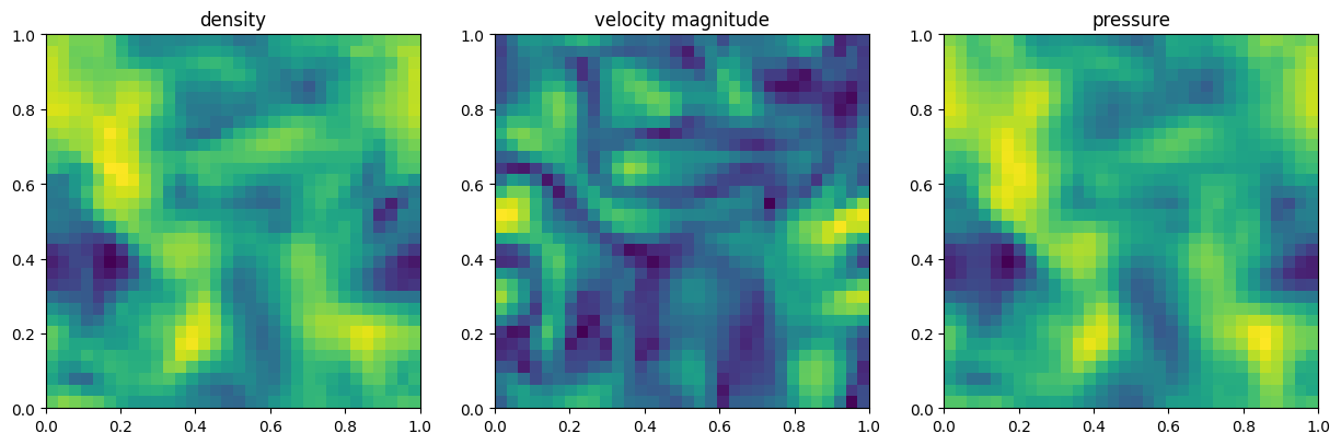
fig, (ax1, ax2, ax3) = plt.subplots(1, 3, figsize=(15, 5))

# equal aspect ratio
ax1.set_aspect('equal', 'box')
ax2.set_aspect('equal', 'box')
ax3.set_aspect('equal', 'box')

z_level = num_cells // 2

ax1.imshow(turb_state[registered_variables.density_index, :, :, z_level].T, origin = "lower", extent = [0, 1, 0, 1], norm = LogNorm())
ax1.set_title("density")

ax2.imshow(jnp.sqrt(turb_state[registered_variables.velocity_index.x, :, :, z_level]**2 + turb_state[registered_variables.velocity_index.y, :, :, z_level]**2 + turb_state[registered_variables.velocity_index.z, :, :, z_level]**2).T, origin = "lower", extent = [0, 1, 0, 1])
ax2.set_title("velocity magnitude")

ax3.imshow(turb_state[registered_variables.pressure_index, :, :, z_level].T, origin = "lower", extent = [0, 1, 0, 1], norm = LogNorm())
ax3.set_title("pressure")

OPTIMAL_BACKEND: using the PALLAS backend (GPU compute capability >= 8.0).
For 3D simulations with periodic boundaries, setting boundary handling to PERIODIC_ROLL and num_ghost_cells to 0 for better performance.
Setting time integrator to RK4_SSP for finite difference solver mode.
RMS velocity: 53.72294235229492 km / s
Turbulent crossing time: 54601.93609289645 yr

Text(0.5, 1.0, 'pressure')

Adapting the target to the total mass in the simulation

total_mass = jnp.sum(turb_state[registered_variables.density_index])
target = target / jnp.sum(target) * total_mass

Adapt the simulation, turn off the turbulent driving

config = config._replace(
    differentiation_mode = BACKWARDS,
    progress_bar = False,
    num_checkpoints = 10,
    turbulent_forcing_config = TurbulentForcingConfig(
        turbulent_forcing = False,
    ),
)

t_final = crossing_time / 2
t_end = t_final.to(code_units.code_time).value
print(t_end)

params = params._replace(
    t_end = t_end,
)

0.9307010712875466

Velocity Optimization

Define the loss

def loss(velocity):

  # set the current velocity
  initial_state = turb_state.at[registered_variables.velocity_index.x].set(velocity[0])
  initial_state = initial_state.at[registered_variables.velocity_index.y].set(velocity[1])
  initial_state = initial_state.at[registered_variables.velocity_index.z].set(velocity[2])

  # integrate in time
  final_state = time_integration(initial_state, config, params, registered_variables)

  # get the final density
  density = final_state[registered_variables.density_index]

  # sum density along z
  projected_density = jnp.sum(density, axis = (2,))
  density_loss = jnp.mean(jnp.square(projected_density - target))
  return density_loss

initial_loss = loss(turb_state[registered_variables.density_index])
print(f"Initial loss: {initial_loss}")

Initial loss: 6.931788084330037e-05

Optimization

current_velocity = jnp.array([
  turb_state[registered_variables.velocity_index.x],
  turb_state[registered_variables.velocity_index.y],
  turb_state[registered_variables.velocity_index.z],
])

# optimizer setup
learning_rate = 5e-2
optimizer = optax.adam(learning_rate)
opt_state = optimizer.init(current_velocity)

# gradient
grad_loss = jax.grad(loss)

best_loss = initial_loss
best_velocity = current_velocity

# optimization
num_steps = 150
for step in range(num_steps):
    grads = grad_loss(current_velocity)
    updates, opt_state = optimizer.update(grads, opt_state)
    current_velocity = optax.apply_updates(current_velocity, updates)

    current_loss = loss(current_velocity)
    print(f"Step {step}: loss = {current_loss}")

    if current_loss < best_loss:
        best_loss = current_loss
        best_velocity = current_velocity

best_state = turb_state.at[registered_variables.velocity_index.x].set(best_velocity[0])
best_state = best_state.at[registered_variables.velocity_index.y].set(best_velocity[1])
best_state = best_state.at[registered_variables.velocity_index.z].set(best_velocity[2])

print("Optimization finished.")

final_loss = loss(best_velocity)
print(f"Final loss: {final_loss}")

Step 0: loss = 3.5333963751327246e-05
Step 1: loss = 0.00010204285354120657
Step 2: loss = 6.9849455030635e-05
Step 3: loss = 2.3276303181773983e-05
Step 4: loss = 1.6590558516327292e-05
Step 5: loss = 2.3357757527264766e-05
Step 6: loss = 1.9768385755014606e-05
Step 7: loss = 1.1353656191204209e-05
Step 8: loss = 8.90491355676204e-06
Step 9: loss = 1.0847567864402663e-05
Step 10: loss = 1.0375842975918204e-05
Step 11: loss = 7.42836891731713e-06
Step 12: loss = 5.602844339591684e-06
Step 13: loss = 5.729825716116466e-06
Step 14: loss = 5.873825102753472e-06
Step 15: loss = 5.0006501624011435e-06
Step 16: loss = 3.912551619578153e-06
Step 17: loss = 3.388764071132755e-06
Step 18: loss = 3.2654656934028026e-06
Step 19: loss = 2.9605257623188663e-06
Step 20: loss = 2.4287976430059643e-06
Step 21: loss = 2.1230530364846345e-06
Step 22: loss = 2.134921260221745e-06
Step 23: loss = 2.125101218553027e-06
Step 24: loss = 1.913773303385824e-06
Step 25: loss = 1.6422769704149687e-06
Step 26: loss = 1.458568135603855e-06
Step 27: loss = 1.3511644283425994e-06
Step 28: loss = 1.274403985007666e-06
Step 29: loss = 1.2302990626267274e-06
Step 30: loss = 1.1591100701480173e-06
Step 31: loss = 9.99183157546213e-07
Step 32: loss = 8.420945505349664e-07
Step 33: loss = 7.867172939768352e-07
Step 34: loss = 7.890991469139408e-07
Step 35: loss = 7.355620255111717e-07
Step 36: loss = 6.213109031705244e-07
Step 37: loss = 5.503325155586936e-07
Step 38: loss = 5.442137762656785e-07
Step 39: loss = 5.25177256349707e-07
Step 40: loss = 4.6535222963939304e-07
Step 41: loss = 4.1930795191547077e-07
Step 42: loss = 4.129633737193217e-07
Step 43: loss = 4.011475880361104e-07
Step 44: loss = 3.5036202916671755e-07
Step 45: loss = 3.0130459549582156e-07
Step 46: loss = 2.9872313689338625e-07
Step 47: loss = 3.149401948121522e-07
Step 48: loss = 2.970867001295119e-07
Step 49: loss = 2.503526275177137e-07
Step 50: loss = 2.1958631180041266e-07
Step 51: loss = 2.1953246687189676e-07
Step 52: loss = 2.234849318938359e-07
Step 53: loss = 2.08795199796441e-07
Step 54: loss = 1.8489228637008637e-07
Step 55: loss = 1.7147468156508694e-07
Step 56: loss = 1.7084548176171666e-07
Step 57: loss = 1.7064630242202838e-07
Step 58: loss = 1.6168256422588456e-07
Step 59: loss = 1.4642927226304892e-07
Step 60: loss = 1.3586669922460715e-07
Step 61: loss = 1.3474775073518686e-07
Step 62: loss = 1.3450733149511507e-07
Step 63: loss = 1.27835022567524e-07
Step 64: loss = 1.1928445076136995e-07
Step 65: loss = 1.1493564500142384e-07
Step 66: loss = 1.1268153343735321e-07
Step 67: loss = 1.0799661254168313e-07
Step 68: loss = 1.0223055824098992e-07
Step 69: loss = 9.928277222570614e-08
Step 70: loss = 9.775791198762818e-08
Step 71: loss = 9.411473911313806e-08
Step 72: loss = 8.974661369620662e-08
Step 73: loss = 8.749366742222264e-08
Step 74: loss = 8.636855142185595e-08
Step 75: loss = 8.41862544120886e-08
Step 76: loss = 8.108459326194861e-08
Step 77: loss = 7.84878011472756e-08
Step 78: loss = 7.688441172604144e-08
Step 79: loss = 7.564958082184603e-08
Step 80: loss = 7.406839586110436e-08
Step 81: loss = 7.209456498458167e-08
Step 82: loss = 7.022363490705175e-08
Step 83: loss = 6.877769465063466e-08
Step 84: loss = 6.758837400866469e-08
Step 85: loss = 6.64261889937734e-08
Step 86: loss = 6.518349948692048e-08
Step 87: loss = 6.386837725358419e-08
Step 88: loss = 6.254024498275612e-08
Step 89: loss = 6.133760166449065e-08
Step 90: loss = 6.045068801086018e-08
Step 91: loss = 5.966807492541193e-08
Step 92: loss = 5.856700369122336e-08
Step 93: loss = 5.734997543527243e-08
Step 94: loss = 5.64559989868485e-08
Step 95: loss = 5.5710724922164445e-08
Step 96: loss = 5.480967146809235e-08
Step 97: loss = 5.393580693180411e-08
Step 98: loss = 5.3266798971662865e-08
Step 99: loss = 5.255078860955109e-08
Step 100: loss = 5.1663683109381964e-08
Step 101: loss = 5.085887622158225e-08
Step 102: loss = 5.023532168024758e-08
Step 103: loss = 4.961028565730885e-08
Step 104: loss = 4.890075544494721e-08
Step 105: loss = 4.821792742859543e-08
Step 106: loss = 4.760592275943054e-08
Step 107: loss = 4.698602396047136e-08
Step 108: loss = 4.6355577154599814e-08
Step 109: loss = 4.5778310919786236e-08
Step 110: loss = 4.522333796330713e-08
Step 111: loss = 4.464411773597021e-08
Step 112: loss = 4.4079669692109746e-08
Step 113: loss = 4.355513993914428e-08
Step 114: loss = 4.304052581005635e-08
Step 115: loss = 4.251577934155648e-08
Step 116: loss = 4.1999523858748944e-08
Step 117: loss = 4.151311117084333e-08
Step 118: loss = 4.1051617216680825e-08
Step 119: loss = 4.058392377714881e-08
Step 120: loss = 4.0113484089943086e-08
Step 121: loss = 3.9672737983664774e-08
Step 122: loss = 3.925774194613041e-08
Step 123: loss = 3.883307186924867e-08
Step 124: loss = 3.840455420345279e-08
Step 125: loss = 3.800047565505338e-08
Step 126: loss = 3.761822142678284e-08
Step 127: loss = 3.723208763517505e-08
Step 128: loss = 3.6843061934632715e-08
Step 129: loss = 3.6471767828061274e-08
Step 130: loss = 3.6112165702206767e-08
Step 131: loss = 3.5754766258833115e-08
Step 132: loss = 3.540193205253672e-08
Step 133: loss = 3.5059620984156936e-08
Step 134: loss = 3.472162646289689e-08
Step 135: loss = 3.4390254199934134e-08
Step 136: loss = 3.406651316595344e-08
Step 137: loss = 3.37453940346677e-08
Step 138: loss = 3.342940857464782e-08
Step 139: loss = 3.312058893811809e-08
Step 140: loss = 3.281883209638181e-08
Step 141: loss = 3.2520269144242775e-08
Step 142: loss = 3.2226129320633845e-08
Step 143: loss = 3.193849096305712e-08
Step 144: loss = 3.1654671772685106e-08
Step 145: loss = 3.137464688052205e-08
Step 146: loss = 3.1099503416953667e-08
Step 147: loss = 3.0829351516104e-08
Step 148: loss = 3.056260311495862e-08
Step 149: loss = 3.029870754289732e-08
Optimization finished.
Final loss: 3.029870754289732e-08

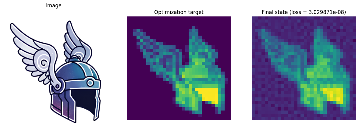
final_state = time_integration(best_state, config, params, registered_variables)

fig, ax = plt.subplots(1, 3, figsize=(15, 5))

ax[0].imshow(original_rgb)
ax[0].set_title("Image")
ax[0].axis("off")

ax[1].imshow(target, cmap="viridis")
ax[1].set_title("Optimization target")
ax[1].axis("off")

ax[2].imshow(jnp.sum(final_state[registered_variables.density_index], axis = (2,)))
ax[2].set_title(f"Final state (loss = {loss(best_velocity):3e})")
ax[2].axis("off")

plt.savefig("overview.png", dpi = 600)

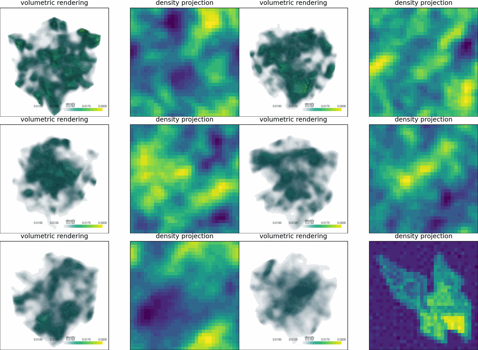
Animation

config = config._replace(
    activate_snapshot_callback = True,
    num_snapshots = 200
)

import os

# create folder for frames
os.makedirs('frames', exist_ok=True)

# empty the folder
for filename in os.listdir('frames'):
  os.remove(os.path.join('frames', filename))

def save_frame(
  time,
  state,
  registered_variables
):

    plot_3D = True

    def plot_slices(density, time):

        print(f"plotting slice at t = {time}")

        if plot_3D:
            fig, (ax1, ax2) = plt.subplots(1, 2, figsize=(8, 4))

            # 3D volumetric rendering in pyvista
            density_3d = np.asarray(density)
            grid = pv.ImageData()
            grid.dimensions = np.array(density_3d.shape) + 1
            grid.cell_data["density"] = density_3d.ravel(order="F")

            plotter = pv.Plotter(off_screen=True, window_size=(700, 700))
            plotter.add_volume(
                    grid,
                    scalars="density",
                    cmap="viridis",
                    clim=(0.01, 0.02),
                    opacity="sigmoid",
                    blending="composite",
                    shade=True,
            )
            plotter.camera_position = "iso"
            volume_img = plotter.screenshot(return_img=True)
            plotter.close()

            ax1.imshow(volume_img)
            ax1.set_title("volumetric rendering")
            ax1.set_xticks([])
            ax1.set_yticks([])

            # projection
            ax2.set_aspect('equal', 'box')
            ax2.set_xticks([])
            ax2.set_yticks([])
            ax2.imshow(np.sum(density_3d, axis = (2,)))
            ax2.set_title("density projection")
        else:
            fig, ax2 = plt.subplots(1, 1, figsize=(4, 4))

            # projection
            ax2.set_aspect('equal', 'box')
            ax2.set_xticks([])
            ax2.set_yticks([])
            ax2.imshow(density)
            ax2.set_title("density projection")

        fig.savefig(
            f"frames/frame{time}.png",
            dpi=150,
            bbox_inches="tight",
            pad_inches=0
        )

        plt.close(fig)

    if plot_3D:
        jax.debug.callback(
            plot_slices,
            state[registered_variables.density_index], time,
        )
    else:
        jax.debug.callback(
            plot_slices,
            jnp.sum(state[registered_variables.density_index], axis = (2,)), time,
        )

final_state = time_integration(best_state, config, params, registered_variables, save_frame)

import imageio.v3 as iio
import os
import re

def get_sorted_frames(directory):
    files = [f for f in os.listdir(directory) if f.endswith('.png')]
    # Extract numerical timestamp from filename (e.g., frame0.123.png -> 0.123)
    # and sort by it
    files.sort(key=lambda f: float(re.search(r'frame([0-9.]+)\.png', f).group(1)))
    return [os.path.join(directory, f) for f in files]

all_frames = get_sorted_frames('frames')

# Read all images into a list
images = [iio.imread(frame) for frame in all_frames]

# Create GIF
gif_path = 'simulation_animation.gif'
iio.imwrite(gif_path, images, duration=int(1000/30))

print(f"GIF created at: {gif_path}")

from IPython.display import Image
Image(filename='simulation_animation.gif')

GIF created at: simulation_animation.gif